Falling into the sun
Recently, I came across a gem of a physics problem, which had the awesome combination of being easy to comprehend, yet being surprisingly difficult to solve.
The problem is thus:
The earth orbits around the sun because it has angular momentum. If we stopped the earth in orbit then let it fall straight towards the sun, then how long would it take to reach the sun in seconds?
Now, I love physics and maths, and I believed that it would be a simple matter to knock this one off. Hah… was I mistaken.
All right… first, I did succeed in finding the answer and it turned out to be worthy of all the trouble. But before I tell you what it is, why don’t you join me in the journey that starts from the first principles and leads to this beautiful result. If you are impatient, just scroll to the bottom for the answer… but if you can hold on to your horses (and don’t mind some mathematics), you might enjoy yourself more.
Ok, lets start.
We want to find out the time taken by an object, ( the earth ), to fall towards a much heavier object, ( the sun ), purely under the force of gravity, given that starts to fall at time from a stationary position a certain distance away. Let us assume that the earth and the sun lie on the axis and at time , let the earth be located at at and the sun at .
We know from Newton’s Law of Gravitation that the force between the earth and the sun is given by
where
- : force in newtons ()
- : gravitational constant :
- : mass of the sun :
- : mass of the earth :
- : distance between earth and sun in meters (changes as earth falls).
- at ,
Also, let be the position of the earth on the , such that, at any given time, is the distance between the earth and the sun. Now, we try to solve this equation to find the time…
Now, we also know that
and we can write
The was one of the key steps which enables us to separate the variables and solve the differential equation. Now,
Separating the variables (moving dx to the right side) and integrating, we get
Performing the integration, we get
where is the constant of integration. We find by using the known condition that at ,
Putting this value of in the equation for ,
If you look closely, you might notice that the above equation is the law of conservation of gravitational potential and kinetic energy. Woohoo… we just derived a conservation law from first principles (Aside : this intermediate result probably keeps popping up in astronomical problems all the time, and was made into a law of it own. I could have used this law right in the beginning to find the velocity at any distance from the sun, but then, I would not have derived the conservation law by myself). Ok… back to the problem.
Moving to the right and variables involving to the left and integrating, we get
This is where I hit another roadblock. The integral on the left side looked harmless enough, but was surprisingly difficult to solve (as we know well enough about integrals… if someone is getting too cocky about their mathematical abilities, give them a random integral, or a partial differential equation to solve). I finally took the help of Wolfram|Alpha to find the indefinite integral of the left side, and was pleasantly surprised that the function did exist (I differentiated it to make sure that it really was the right answer, and you should try it too. Just like in the spy movies… trust no one. In this case, not even yourself… so check your answer twice, and get it peer reviewed). We now have the following:
At both and , the term inside the parentheses contains a division by zero. Usually, that is disastrous for a solution. However, in this case, its not too bad as is well defined. And to know whether the division by zero leads to a or a , we need to evaluate the LHS at and :
The term equals at both and
Putting the LHS and RHS together, we get
Rearranging the variables around, we finally get
As often happens in interesting problems, we have journeyed from a simple equation (newton’s law) to terrible looking intermediate results, divisions by zero, and challenging integrals… which all finally canceled out to give a simple answer.
Wait… there is a in the answer!! How in the frigging cosmos did make its way into the answer. Well, we can go back and look at where it exactly came in… through the and , which basically means that it popped out from a couple of singularities. It might also have something to do with the periodic oscillation that the earth might have experienced were it not going to be evaporated on contact with the sun. This is as close to magic as we get in mathematics, and yet another beautiful example of unexpected places where shows up.
Now that we have done all the hard work of finding the general solution, its time to put in the values to get the figure of…
or about 2.1 months.
All this is excellent but I also love programming. Its time to test this analytical solution with a numerical calculation.
I wrote a small python program to calculate the time by simulating the acceleration, velocity and position of the earth as it falls towards the sun. I have also plotted a graph denoting the distance of earth from the sun vs time.
%matplotlib inline

# calculate time for earth to fall into sun...
from math import sqrt
from time import time

# physical constants/values
G = 6.67384e-11 # gravitational constant
MS = 1.98855e30 # mass of sun
esd = 149597870700.0 # earth-sun distance in meters

# program variables
n = 1000000
myconst1 = (G*MS*n*n)/(esd*esd)
myconst2 = esd/n

def getA(k):
    """ acceleration at distance (esd*k/n) from sun"""
    ak = myconst1/pow(n-k,2)
    return ak

def getV(v, a, t):
    """ velocity at distance (esd*k/n) from sun"""
    vk = v + a*t
    return vk

def getVAT(k, vold, aold, told):
    """ time to get from position (esd*k/n) to (esd*(k+1)/n)"""
    vk = getV(vold, aold, told)
    ak = getA(k)

    tk = (sqrt(vk*vk + 2*ak*myconst2) - vk)/ak
    return vk, ak, tk

stime = time()
sts, v, a, t = 0, 0, 0, 0
plotValues = []
for x in range(n):
    v, a, t = getVAT(x, v, a, t)
    sts += t
    if x % 5000 == 0:
        plotValues.append((sts, n - x))
plotValues.append((sts, n-x-1))

print "Travel time = %.2f seconds\nDays = %5.3f"%(sts, sts/(60.0*60*24))
print "Computation time = %5.4f seconds"%(time() - stime)
Travel time = 5578753.47 seconds
Days = 64.569
Computation time = 1.8074 seconds
Here’s the plot of earth’s approach towards the sun…
import matplotlib.pyplot as plt
xvals = [sts for sts, x in plotValues]
yvals = [149.597870*x for sts, x in plotValues]
plt.xlabel("Travel time (seconds)")
plt.ylabel("Distance between earth / sun (km)")
plt.plot(xvals, yvals)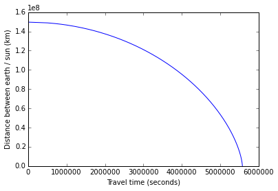
Comments